Pivot tables are one of the most powerful features in Excel and they can make your data easy to use and manage with a minimum of effort. In this tutorial you are going to learn how to create a pivot table in Excel 2013.
- join us on Facebook
Step # 1 -- Finding the Place for the Table
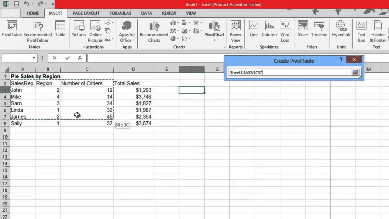
First of all you are going to want to have some data already in your sheet. As you can see here we have some fictional information about the sales figures for some items in a store. Click into any cell near to this sheet where you would like your pivot table to appear.
Step # 2 -- Creating the Pivot Table
Click on the Insert tab in the ribbon at the top and then click the Pivot Table icon on the left. A dialog box will appear and you are going to need to select a range for your pivot table. Drag your mouse over the area that you want to take the data from (here that is our entire table) and then click OK.
Step # 3 -- Selecting the Fields
You are now going to need to set up the fields for the pivot table. Here we will choose to include all the options, but you can really just select what you need for your table. As you select or deselect them, different options will appear. As you will be able to see the pivot tool is remarkably good at presenting the data you need and is a very powerful tool.
You now know how to create pivot table in Excel 2013
Deke: Spent almost an hour, watching videos and reading articles on how to create pivot tables, only to realize I still didnt know what I was doing. I watched your 1 minute video and Ive got it. Awesome job! Thanks so much for getting right to the point and leaving out the fluff. Date: 2023-07-08